
Numbers in computers can only be represented by a fixed number of digits. The predominant number type in Finite Element Method (FEM) software packages is Double-Precision, which is 8 bytes in size. This gives about 15 digits of accuracy. However, during the solution of FEM equations, numerical difficulties or errors may be encountered in certain modeling scenarios due to truncation and round-off errors. The introduction of the Quad-Precision number type, 16 bytes in size providing about a 34-digit accuracy, can reduce FEM solution errors. The author presents a few examples to illustrate the differences in using Double Precision and Quad Precision numbers.
A few types of errors are associated with finite element/structural analysis programs.
- Input/output errors: user input mistakes while entering input data or misinterpreting program results.
- Modeling errors: assumptions made in the formulation of mathematical models (e.g., using elastic material properties for concrete).
- Discretization errors: using discretized finite element models for continuous mathematical models (e.g., using straight elements to model a curved edge).
- Solution errors: numerical errors during the process of numerical solutions of finite element equations.
Although all the above errors are important, this article focuses on solution errors.
Finite element solutions boil down to solving a system of linear equations:
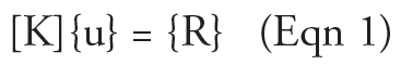
where [K] is the global stiffness matrix, {u} is the displacement vector, and {R} is the load vector.
During the solution of the above system of linear equations, truncation errors, round-off errors, and accumulation errors can be experienced. This article illustrates these errors through examples.
Basic Number Concept in Computers
Numbers, like any other information in computers, are represented by bytes. A byte consists of eight bits. One bit can represent 2 states (on and off), two bits can represent 22 states, and so on. Therefore, a byte can represent 28 = 256 states. There are two main floating-point (non-integral) number types in computers: 4-byte (or 32-bit) single-precision type and 8-byte (or 64-bit) double-precision type.
As we all know, infinite numbers exist between any two different numbers. So how can we represent numbers accurately with a limited number of bits or bytes in a computer? The answer is we cannot. We can only represent numbers in a computer by approximation. For the 32-bit single-precision number type, we generally use 1 bit to represent signs (positive or negative), 8 bits to represent exponents, and 23 bits to represent actual digits. Since 223 = 8388608, it can be said that a single-precision number has an accuracy of about 7 significant digits. For the 64-bit double-precision number type, we generally use 1 bit to represent signs, 11 bits to represent exponents, and 52 bits to represent actual digits. Since 252 = 4.5 E15, a double-precision number could be viewed as having an accuracy of about 16 significant digits.
The concept of significant digits can have unexpected results in software computations. For example, if we have three double-precision numbers x = 1.234e18; y = 0.1; z = x + y; both x and z will still equal to 1.234e18. A more serious issue is that the number y / (z–x) yields infinity instead of 1. In today’s finite element programs, double precision is the predominant number type used in their implementations and is sufficient in most cases. However, double precision may not be accurate enough in some uncommon cases.
Truncation and Round-Off Errors
Suppose we have the following system of equations in matrix form [K]{u} = {R}
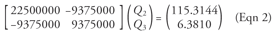
Solving the equations by the Gauss elimination method using 15 significant digits yields the following “accurate” solution:
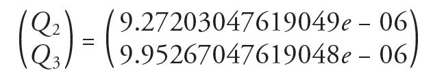
Now pretend that a computer can only represent each number accurately to 3 significant digits. Then the original system of equations Equation 2 becomes
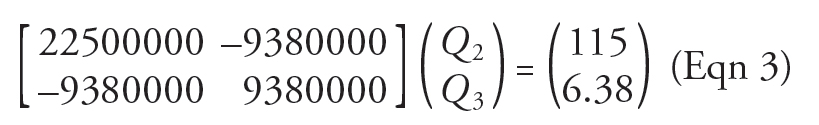
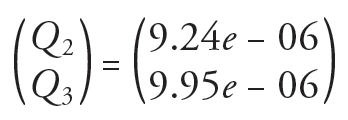
Here, we chopped off the stiffness matrix and load vector terms from Equation 2 to 3 significant digits. Therefore, we have a truncation error introduced in Equation 3 even if we solve the equations accurately with 15 significant digits. If we continue to solve the equations with 3 significant digits in each arithmetic step, additional round-off errors are introduced, and the following solution results:
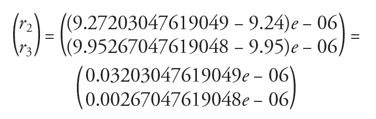
The accumulated truncation and round-off errors, r2 and r3, for displacements Q2 and Q3 are:
A Simple Structural Model
In forming the global stiffness [K] in Equation 3, each stiffness term Kij is calculated by adding the relevant stiffness terms of all elements connected to the associated degree of freedom. For simplicity’s sake, assume Kij comes from two elements with the relevant element stiffness terms k1 and k2; thus, Kij = k1 + k2. If k1 is much smaller than k2 (or vice versa), significant information is irrevocably lost due to truncation error. As a result, the solution for displacements may be inaccurate, incorrect, or impossible.

The following simple structure consists of two 10-foot one-dimensional elements (Figure 1) and is subjected to an axial load of 1 kip at the tip. The material’s modulus of elasticity, E, equals 29000 kips per square inch (ksi). The first element (B1) has a cross-sectional area of 0.0001 inches2. We vary the cross-sectional area of the second element (B2) using 0.0001, 0.01, 1, 100, 10000, 1e+06, 1e+10, 1e+12, and 1e+14 inches2.
The results in Table 1 are from a Real3D software program using double-precision arithmetic.
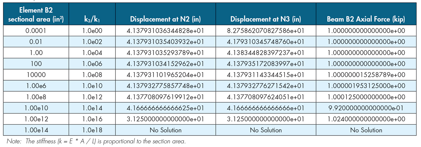
The results deteriorate as the stiffness mismatch between the two elements becomes larger. The result becomes inaccurate when k2/k1 = 1.00e10 / 0.0001 = 1.0e14, unreliable when k2/k1 = 1.00e12 / 0.0001 = 1.0e16, and unattainable when k2/k1 = 1.00e14/0.0001 = 1.0e18. This behavior is expected due to the double-precision number having an accuracy of about 16 significant digits.
A Cantilever Beam Modeled with Multiple Segments
Numerical difficulties may also arise due to the accumulation of round-off errors, primarily when a model consists of a large number of elements. The following cantilever beam example is modeled with multiple segments of equal lengths, thus without any element stiffness mismatches.
A 100-inch-long horizontal cantilever beam is subjected to a vertical point load of -10,000 pounds (lbs.) at the tip.
Material properties: E = 2.9e7 pounds per square inch (psi), Poisson’s ratio, ν = 0.3
Section properties: a moment of inertia I = 200 inches^4
Model the beam with 1; 1,000; 10,000; 20,000; and 50,000 members or segments.
Also, beam shear deformations are not considered.
The displacement and rotation at the tip of the beam may be calculated by hand as follows:
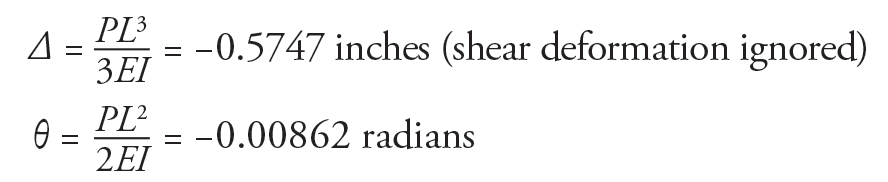
The results in Table 2 are from the Real3D software program using a double-precision solver and a quad-precision solver.
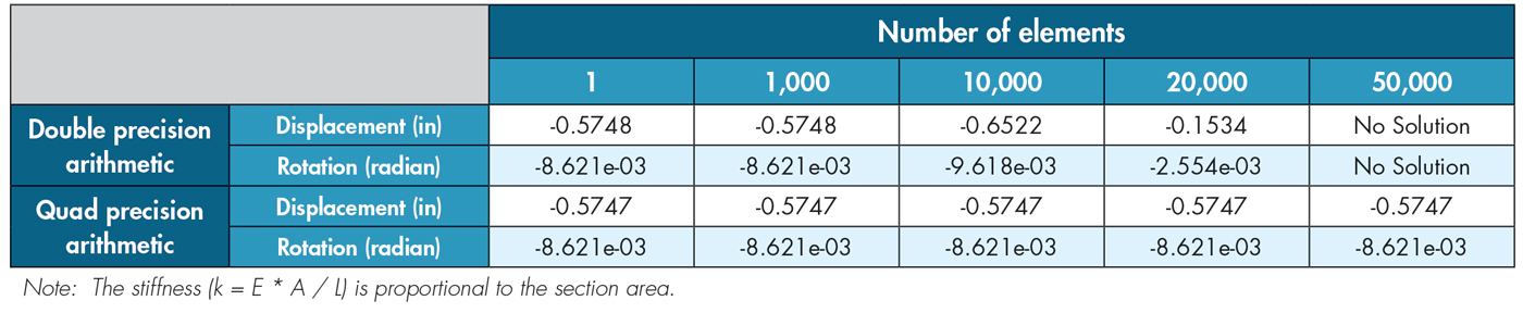
This example is probably the simplest structural model that can be solved by either hand or an analysis program. However, it could be a very challenging numerical problem, as shown. The standard double-precision solver tends to deteriorate in solution accuracy as the number of elements increases. In the example, the solver becomes unstable after 10,000 elements. For the model with 50,000 elements, some diagonal terms in the global stiffness matrix become negative during the factorization process due to round-off errors. As a result, the solver has to terminate, and the solution is no longer obtainable. No results are actually better than wrong results. You are encouraged to solve this model with your familiar structural analysis software!
The quad precision solver is much more accurate and stable. The quad-precision number type uses 16 bytes or 128 bits with 1 bit to represent signs, 15 bits to represent exponents, and 112 bits to represent actual digits. It has an accuracy of about 34 significant digits. (Can you figure out why? It’s because 2^112 = 5.2E33). Therefore, it is more tolerant to round-off error accumulation. Consistent and correct results from the quad precision solver demonstrate its superior accuracy for up to 50,000 or more elements for this example.
A Continuous Beam with Large Stiffness Differences
The following 700-foot continuous bridge (Figure 2) is discretized into multiple segments of different lengths: 0.3, 9.7, 20@10, 0.3, 9.7, 27@10, 0.3, 9.7, 20@10 feet. Each segmented beam is subjected to a uniform load of -0.9 kip/ft in the global Z-direction.

Material: E = 30457.9 ksi, ν = 0.25
Sections: Izz = 2.40251e + 06 in4 , Iyy = 619965 in4,
J = 2.40251e+06 in4, A = 255.441 in2, Ay = Az = 0.0 in2
Support conditions:
@Node 2: restrained in Dx, Dy, Dz, and Dox degrees of freedom
@Node 24: restrained in Dy, Dz, and Dox rotational degrees of freedom. There is a large support settlement of 14.5107 inches in the Z direction.
@Node 53: restrained in Dy, Dz, and Dox degrees of freedom
The results in Table 3 are from the Real3D software program using the double-precision skyline matrix solver, double-precision sparse matrix solver, and quad-precision skyline matrix solver (see Note 1).
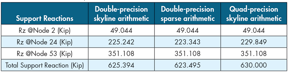
The total support reaction in the Z direction should be 700 ft * 0.9 kip/ft = 630 kips. However, as shown, both the double-precision skyline solver and sparse solver give an inaccurate support reaction at Node 24 that is reflected in the total support reaction. The reasons for this inaccuracy are due to the following:
- There is a significant stiffness variation between adjacent beams at the support.
- The Real3D software program uses a penalty approach (see Note 2) to enforce support restraints when constructing global stiffness matrices.
- The support settlement (load value) is large.
These reasons result in significant truncation and round-off errors with double-precision arithmetic. On the other hand, the quad precision arithmetic yields an accurate support reaction at Node 24.
*Note 1: The skyline and sparse matrix refer to how the global stiffness matrix is stored. The sparse matrix solver generally uses much less memory and runs faster than the skyline matrix solver. Note 2: The penalty approach uses springs with large stiffness values to model supports. This approach is popular among structural analysis software implementations due to its simplicity and intuitiveness.
Rigid Diaphragm Modelling
In modeling rigid diaphragms such as a concrete floor in a frame, master-slave (where slave nodes are constrained to follow a master node) degrees of freedom DX, DZ, and DOY (rotation about the global Y axis) could be used, assuming Y is the vertical axis. This is mathematically imposing constraint equations in the global stiffness matrix. However, this approach may not be ideal since DX and DZ are not equal for all the nodes on the diaphragm plane when subjected to unsymmetrical loading.
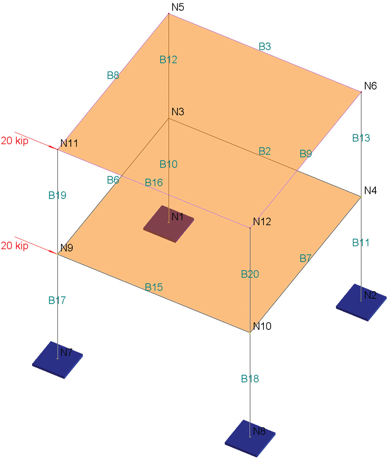
A more reasonable way to model rigid diaphragms (Figure 3) is to add fictitious members with very large in-plane stiffnesses relative to the model’s actual members. The fictitious members must be interconnected with all the nodes on the diaphragm plane. These fictitious members can then be assigned large material properties and in-plane sectional properties based on those of actual members and a large stiffness multiplier (say 1.0e4). This ensures the rigid in-plane diaphragm action. Some structural software programs in the market implement this feature automatically.
A potential problem with the second approach is using a large stiffness multiplier in the double-precision solver. It artificially increases the mismatch of member stiffness terms, thus increasing the likelihood of numerical difficulties during the solution. With quad precision, this problem can be easily avoided.
Tips for Detecting and Minimizing Solution Errors
As the previous examples show, structural analysis software programs may not always yield accurate results. There are some inherent errors associated with constructing and solving systems of equations. In certain situations, these errors may become intolerable. Of course, structural analysis software, like any other software program, may contain defects (i.e., software bugs). A good structural engineer should not blindly trust software results.
If possible, a suitable software program should warn users when numerical difficulties or errors are encountered during a solution. A useful measure is the number of significant digits lost during the analysis solution. It can be computed based on the diagonal decay ratio (ri) as defined below.
ri = Kii / Pii
where Kii is the original diagonal coefficient of the global stiffness matrix, and Pii is the reduced value of Kii just before it is used for back-substitution. The number of significant digits lost is about log10(ri). For example, if ri is 108, then 8 digits are lost. The results given by double-precision solvers may be unreliable if 12 or more significant digits are lost during the solution process.
The following are a few tips to minimize solution errors when using structural analysis software:
a) Avoid large stiffness differences between adjacent elements. For example, for one-dimensional frame members, the member lengths should not vary too much; for two- or three- dimension finite elements such as shells or brick elements, the element sizes and shapes should be close or nearly the same.
b) Use master-slave degrees of freedom if possible (e.g., use displacement constraints for rigid beams in two-dimensional frames).
c) Use higher precision (e.g., quad-precision) number arithmetic if needed. If your software vendor does not currently support it, ask for it. It should be noted that quad-precision numbers take twice as much memory as double-precision numbers. It is also significantly slower due to the lack of direct hardware support and extra calculations.
d) Never use any finite element software programs that use single-precision arithmetic in their solver. This may be a problem in some older structural software programs when computer memory was a premium. Single-precision number types should not be used in finite element implementations.
e) Pay attention to software errors or warning messages such as significant digits lost during factorization of global stiffness matrices.
f) Check if the summation of support reactions is equal to the total load. Since finite element implementations are displacement-based, if displacements are unreliable due to unstable solutions, all other results, such as support reactions, are unreliable.■
References
K.J. Bathe, Finite Element Procedures, Prentice-Hall, Inc., 1996
Chandrupatla and Belegundu, Introduction to Finite Elements in Engineering, Pearson, 4th ed.
R.C. Cook and D.S. Malkus and M.E. Plesha, Concepts and Applications of Finite Element Analysis, 3rd ed., John Wiley & Sons, Inc., 1989